Cost Optimization & Performance Tuning in MLOps

Welcome

Hey — I'm Aviraj 👋

Mastering cost optimization and performance tuning in MLOps empowers us to build efficient, scalable ML pipelines that maximize ROI while minimizing resource waste. It ensures models run faster, cheaper, and more reliably in production, directly impacting business value and user experience.

🔗 30 Days of MLOps

📖 Previous => Day 27: Model Deployment with Serverless Architectures

📚 Key Learnings

Understand where costs accumulate in the ML lifecycle (data storage, compute, training, inference, monitoring)
Learn performance bottleneck detection in data processing, training, and serving
Explore cloud-specific cost optimization strategies for AWS, GCP, and Azure
Implement model optimization techniques (quantization, pruning, distillation)
Learn inference optimization (batching, caching, hardware acceleration)

🧠 Learn here

Cost Accumulation in the ML Lifecycle

1. Data Storage

Where costs come from:

Raw Data Storage: Storing large volumes of structured and unstructured data (e.g., images, videos, logs) in cloud storage services (e.g., Amazon S3, Google Cloud Storage, Azure Blob).
Versioned Datasets: Maintaining multiple versions for reproducibility (e.g., DVC, Delta Lake) increases storage consumption.
Backup & Archival: Long-term storage and compliance-related backups.

Cost factors:

Storage size (GB/TB) and class (standard, infrequent access, archive)
Data replication across regions for high availability
Egress fees when moving data between cloud providers or regions

2. Compute

Where costs come from:

ETL & Preprocessing: Running compute-heavy data transformations
Feature Engineering: Generating and aggregating large-scale features
Model Training & Evaluation: GPU/TPU clusters, high-memory CPU instances

Cost factors:

On-demand vs. spot/preemptible instances
Instance type (CPU, GPU, TPU) and runtime
Idle compute due to poor scheduling

3. Training

Where costs come from:

Experimentation Cycles: Multiple iterations of hyperparameter tuning and architecture exploration
Distributed Training: Scaling to multiple nodes for large datasets
Storage for Model Checkpoints: Intermediate model saves during training

Cost factors:

Number of experiments and trial durations
Use of managed ML services (e.g., SageMaker, Vertex AI, Azure ML) vs. self-hosted clusters
Inefficient model architectures leading to excessive compute needs

4. Inference

Where costs come from:

Real-time Serving: Keeping models in memory with low-latency APIs
Batch Predictions: Periodic large-scale inference jobs
Autoscaling: Scaling inference services during peak demand

Cost factors:

Model size and memory footprint
Request volume and throughput requirements
Latency SLAs that require high-performance compute

5. Monitoring

Where costs come from:

Metrics Collection: Storing prediction logs, latency metrics, and feature distributions
Data Drift & Model Drift Detection: Continuous statistical checks on incoming data
Alerting & Dashboards: Real-time monitoring pipelines

Cost factors:

Log retention duration
Frequency of monitoring checks
Use of third-party monitoring tools vs. in-house solutions

Key Cost Optimization Strategies

Use tiered storage (standard, infrequent, archive) for different data needs
Implement spot/preemptible instances for non-critical workloads
Use early stopping and smaller model architectures to reduce training costs
Deploy model compression techniques for cheaper inference
Set log retention policies and optimize monitoring granularity

Performance Bottleneck Detection in ML Systems

Performance bottlenecks in Machine Learning (ML) workflows can significantly slow down execution, increase costs, and degrade the end-user experience. Detecting them early in data processing, model training, and serving stages is key to building efficient ML pipelines.

1. Bottleneck Detection in Data Processing

Symptoms:

Long ETL job runtimes
Delays in data availability for training
High I/O wait times

Common Causes:

Inefficient data formats (e.g., CSV vs. Parquet/ORC)
Unoptimized joins or aggregations in distributed processing (e.g., Spark, Dask)
Data shuffling across network

Detection Methods:

Profiling tools: Apache Spark UI, Dask Dashboard
I/O metrics: CloudWatch, Prometheus node exporter
Data pipeline tracing: OpenTelemetry instrumentation

Quick Wins:

Switch to columnar formats
Push down filters and projections
Increase parallelism in ETL jobs

2. Bottleneck Detection in Model Training

Symptoms:

Underutilized GPUs/TPUs
Long training epochs
Delays between iterations

Common Causes:

Data loading bottlenecks (slow disk or network reads)
Large batch sizes causing memory thrashing
Inefficient model architectures or unoptimized code

Detection Methods:

GPU/CPU utilization monitoring: nvidia-smi, gpustat, cloud metrics
Data pipeline profiling: TensorFlow tf.data profiler, PyTorch profiler
Code profiling: cProfile, Pyinstrument

Quick Wins:

Use prefetching and data caching
Optimize model graph execution
Apply mixed precision training

3. Bottleneck Detection in Model Serving

Symptoms:

High inference latency
Low throughput despite high resource allocation
Autoscaling triggers too frequently

Common Causes:

Heavy model files and slow loading
Inefficient serialization/deserialization
Synchronous processing for parallelizable tasks

Detection Methods:

Load testing: Locust, k6, Apache JMeter
Tracing & profiling: Jaeger, OpenTelemetry
Application performance monitoring (APM): New Relic, Datadog

Quick Wins:

Use model quantization or pruning
Keep model loaded in memory (warm starts)
Batch requests for high-throughput scenarios

Unified Best Practices for Bottleneck Detection

Implement end-to-end observability using tracing + metrics
Establish baseline performance metrics and compare periodically
Automate alerts for performance degradations
Use synthetic workloads to simulate peak conditions

Cloud-Specific Cost Optimization Strategies

1. AWS (Amazon Web Services)

Key Cost Optimization Strategies:

Right-Sizing EC2 Instances: Use AWS Compute Optimizer to identify underutilized or over-provisioned instances. Leverage instance families optimized for workload type (e.g., C for compute, R for memory).
Spot and Savings Plans: Use EC2 Spot Instances for non-critical, fault-tolerant workloads. Purchase Savings Plans or Reserved Instances for predictable workloads.
S3 Storage Class Optimization: Migrate infrequently accessed data to S3 Infrequent Access or Glacier. Enable S3 Lifecycle Policies to automate tiering and deletion.
Lambda Cost Controls: Optimize memory and execution time. Use provisioned concurrency only when necessary.
EBS Volume Management: Delete unattached volumes. Use gp3 volumes instead of gp2 for better performance per dollar.
Data Transfer Cost Reduction: Use CloudFront for content delivery. Keep services in the same AWS region to avoid inter-region transfer fees.

2. GCP (Google Cloud Platform)

Key Cost Optimization Strategies:

Committed Use Discounts (CUDs) and Sustained Use Discounts: Commit to resource usage for 1–3 years for substantial discounts.
Preemptible VMs: Run non-critical workloads on preemptible VMs for up to 80% savings.
Cloud Storage Class Optimization: Use Nearline or Coldline for archival data. Enable Object Lifecycle Management for auto-tiering.
BigQuery Cost Controls: Use table partitioning and clustering to reduce scanned data. Monitor queries to avoid unnecessary full-table scans.
Kubernetes Cost Efficiency: Enable node auto-provisioning. Use GKE Autopilot for small workloads.
Data Transfer Savings: Keep workloads within the same region/zone. Use Cloud CDN for content delivery.

3. Azure (Microsoft Azure)

Key Cost Optimization Strategies:

Azure Reservations and Savings Plans: Reserve VMs, SQL DB instances, or Cosmos DB capacity for 1–3 years.
Azure Spot VMs: Use for batch, stateless, and fault-tolerant workloads.
Blob Storage Tiering: Move infrequently accessed data to Cool or Archive tiers. Use Lifecycle Management rules for automation.
Azure Monitor & Advisor: Review cost recommendations regularly. Identify and remove idle or underutilized resources.
Serverless Cost Control: Optimize Azure Functions' execution time. Implement event filtering to avoid unnecessary triggers.
Network Cost Optimization: Use Azure Front Door or CDN for data delivery. Co-locate services in the same region.

Inference Optimization

Optimize latency, throughput, and cost per request by combining smart batching, caching, and hardware acceleration.

Outcomes & Metrics

Track these always-on KPIs:

p50/p95/p99 latency (ms)
Throughput (req/s, tokens/s)
Cost per 1k requests (infra + egress)
GPU/CPU utilization (%), SM occupancy (GPU)
Batch efficiency = (actual batch size / max batch size)
Cache hit ratio (overall, hot-path)

Useful relation: Little's Law → L = λ × W (in-system requests = arrival rate × latency). Batching increases W slightly to reduce cost/raise throughput; keep SLOs honest.

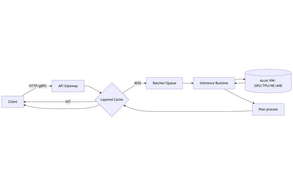
1) Batching

Batching boosts device utilization by amortizing overhead across multiple requests.

Patterns:

Static Batching: Fixed max_batch_size. Simple but may add tail latency at low QPS.
Dynamic/Micro-Batching: Collect requests for a short max batch delay (e.g., 1–10 ms) to build batches opportunistically.
Sequence Batching (Triton): Keep request order for stateful models.
Token/Window Batching (LLMs): Batch by prompt+decode tokens with paged attention/kv-caching.

Tuning Knobs:

max_batch_size, max_queue_delay_ms (a.k.a. preferred_batch_size & max_queue_delay_microseconds in Triton)
Concurrency/workers per model instance (e.g., TorchServe default_response_timeout, batch_size, max_batch_delay)
Warmup: JIT/TensorRT engines and load models before traffic; pre-create CUDA contexts

Pseudocode (Python micro-batcher):

# Simplified micro-batcher: collects requests for up to MAX_DELAY_MS or until MAX_BATCH
Q, MAX_BATCH, MAX_DELAY_MS = [], 32, 5
while True:
    start = now()
    while len(Q) < MAX_BATCH and (now()-start).ms < MAX_DELAY_MS:
        Q += recv_new_requests_nonblocking()
    batch = Q[:MAX_BATCH]; Q = Q[MAX_BATCH:]
    if batch:
        outputs = model(run_stack(batch))
        for r, o in zip(batch, outputs): r.respond(o)

Tips:

Start with max_queue_delay_ms = 2–5 for vision/NLP; 10–30 for LLM token batching; validate SLOs
Prefer larger, fewer batches on GPUs; many small kernels underutilize SMs
Use pinned host memory + async H2D/D2H copies; overlap data transfers with compute

2) Caching

Reduce repeated work on hot inputs/embeddings.

What to Cache:

Preprocess features (tokenized text, resized/normalized images)
Embeddings for retrieval and reranking
Model outputs for idempotent queries (e.g., classification, reruns)
KV-cache for LLM decoding

Layers:

Client/Edge: CDN, Service Worker
API Layer: Reverse proxy (NGINX, Envoy) with cache_key from request hash
App Layer: Redis/Memcached (LRU/LFU), sharded by consistent hashing
Model Layer: In-process LRU (e.g., functools.lru_cache), framework-native KV-cache

Policy:

TTL: Seconds–hours for deterministic models; version cache keys with model_id@sha
Invalidation: On model retrain/deploy; use write-through for freshness
Admission: Cache only items above size/latency thresholds to avoid thrash

Example Cache Key:

cache_key = sha256(model_version + serialize(features, stable=True))

Targets: Aim for >80% hit ratio on hot endpoints; measure tail latency impact from misses.

3) Hardware Acceleration

Map models to best-fit hardware & runtimes.

Runtimes & Compilers:

TensorRT (NVIDIA), ONNX Runtime (EPs: CUDA, TensorRT, OpenVINO, DirectML), XLA (TPU), TVM/TorchInductor, OpenVINO (Intel), Core ML/Metal (Apple ANE), AWS Neuron (Inferentia/Trn1)

Device Picks:

CNN/ViT, general DL: NVIDIA GPUs (A10/A100/L4/H100) w/ TensorRT or ORT-TensorRT
Transformers/LLMs: H100/L40S; for cost efficiency consider L4 + quantization (INT8/FP8)
CPU-only: Use OpenVINO or ORT-CPU + INT8 for classic NLP/CV
Cloud ASICs: TPU v5e/v5p (GCP), Inferentia2/Trn1 (AWS)

Deployment Servers:

Triton Inference Server: Multi-model, dynamic batching, decoupled I/O
TorchServe / TF Serving: Straightforward single-framework serving

Tuning:

Build static engines (TensorRT) with optimal profiles for input shapes
Use mixed precision (FP16/BF16/FP8) when accuracy permits
Pin NUMA/CPU affinity; isolate IRQs; enable IOUring for high I/O

Kubernetes & Autoscaling

KEDA/HPA on QPS/lag/queue depth; define separate SLOs for cold vs warm paths
Pod resources: set requests=limits for GPUs; avoid noisy neighbors
Model sharding: by tenant/model_id to improve cache locality
Node pools: dedicated GPU pools (spot for batch, on-demand for RT)

Load Testing & Profiling

Tools: k6, Locust, vegeta for HTTP; Triton perf_analyzer; nsys, nvprof, torch.profiler, tf.profiler

Method: Fixed RPS steps → soak → spike. Record utilization, queue delay, batch size distribution.

Report: Compare latency/throughput vs batch size, cost/1k req, and hit ratios.

Troubleshooting Checklist

Low GPU util? → Increase batch size, enable async D2H/H2D, fuse ops, enable mixed precision
High p99? → Reduce max queue delay, enable priority lanes, separate real-time from batch
Cache thrash? → Raise cache size, switch to LFU, tighten admission/TTL
Engine warmup spikes? → Preload weights, run warmup inits on deploy, keep min replicas > 0

Configuration Examples

Triton (config.pbtxt):

name: "resnet50"
max_batch_size: 64
input: [{ name: "INPUT__0", data_type: TYPE_FP16, dims: [3,224,224]}]
output: [{ name: "OUTPUT__0", data_type: TYPE_FP16, dims: [1000]}]
dynamic_batching { preferred_batch_size: [8,16,32] max_queue_delay_microseconds: 5000 }
instance_group [{ kind: KIND_GPU, count: 2 }]

TorchServe (config.properties):

inference_address=http://0.0.0.0:8080
model_store=/models
load_models=resnet.mar
batch_size=32
max_batch_delay=5
number_of_netty_threads=64

ONNX Runtime (Python):

import onnxruntime as ort
sess = ort.InferenceSession("model.onnx", providers=["TensorrtExecutionProvider","CUDAExecutionProvider"])
# Warmup
for _ in range(10): sess.run(None, {"input": warmup_batch})

🔥 Challenges

Use AWS/GCP/Azure billing tools to find your top 3 cost drivers
Compress a model with quantization and measure the reduction in inference latency and cost
Run inference in batch mode and compare cost vs. per-request mode
Deploy two versions of your model: full-precision and quantized, and run A/B testing to monitor accuracy vs. cost trade-offs
Create a cost-performance dashboard using Grafana + Prometheus to track:
- Inference latency
- Throughput (req/sec)
- Cost per request
Enable autoscaling for an ML inference service

Navigation

← Previous: Day 27 Roadmap Next: Day 29 →